Using Logistic to solve Classification Problems
The Logistic task solves classification problems according to the logistic regression approach, i.e. by approximating the probabilities associated with the different classes through a logistic function:
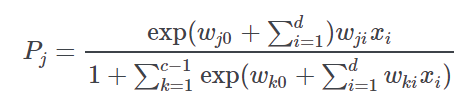
where
c is the number of output classes
j is the index of the class, ranging from 1 to c−1,
d is the number of inputs and
𝓌ji is the weight for class j and input i .
The probability for the c -th class is obtained as

The optimal weight matrix 𝓌ji is retrieved by means of a Maximum Likelihood Estimation (MLE) approach that makes use of the Newton-Raphson procedure to find the minimum of the log-like function.
The output of the task is the weights matrix 𝓌ji, which can be employed by an Apply Model task to perform the Logistic forecast on a set of examples.
Prerequisites
you must have created a flow;
the required datasets must have been imported into the flow;
the data used for the analysis must have been well prepared;
a single unified dataset must have been created by merging all the datasets into the flow.
Additional tabs
the Results tab, where statistics such as the execution time, number of attributes etc. are displayed.
the Coefficients tab, where the coefficients matrix weight vector 𝓌ji relative to the Logistic approximation is shown. Each row corresponds to an output class whereas columns are relative to a single input attributes.
Procedure
Drag the Logistic task onto the stage.
Connect a task, which contains the attributes from which you want to create the model, to the new task.
Double click the Logistic task.
Drag and drop the input attributes, which will be used for regression, from the Available attributes list on the left to the Selected input attributes list.
Configure the options described in the table below.
Save and compute the task.
Logistic options | |
Parameter Name | Description |
|---|---|
Selected input attributes (drag from available attributes) | Drag and drop the input attributes you want to use to form the model leading to the correction classification of data. |
Normalization of input variables | The type of normalization to use when treating ordered (discrete or continuous) variables. Possible methods are:
Every attribute can have its own value for this option, which can be set in the Data Manager task. These choices are preserved if Attribute is selected in the Normalization of input variables option; otherwise any selections made here overwrite previous selections made.
Normalization types For further info on possible types see Advanced Attributes' Management in the Attribute Tab. |
Output attribute (response variable) | Select the attribute which will be used to identify the output. |
P-value confidence (%) | Specify the value of the required confidence coefficient. |
Weight attribute | If specified, this attribute represents the relevance (weight) of each sample (i.e., of each row). |
Regularization parameter | Specify the value of the regularization parameter which is added to the diagonal of the matrix. |
Initialize random generator with seed | If selected, a seed, which defines the starting point in the sequence, is used during random generation operations. Consequently, using the same seed each time will make each execution reproducible. Otherwise, each execution of the same task (with same options) may produce dissimilar results due to different random numbers being generated in some phases of the process. |
Aggregate data before processing | If selected, identical patterns are aggregated and considered as a single pattern during the training phase. |
Append results | If selected, the results of this computation are appended to the dataset, otherwise they replace the results of previous computations. |


Example
The following example uses the Adult dataset.
Description | Screenshot |
|---|---|
Leave the remaining options with their default values and compute the task. |  |
Once computation has completed, in the coefficients tab we have a single row containing the coefficients relative to the output class In a case with c>2 output classes, the weight matrix contains c−1 rows each containing the coefficients relative to an output class. The probability of the last class is obtained as  |  |
The Results tab contains a summary of the computation. Then add an Apply Model task to forecast the output associated with each pattern of the dataset. | 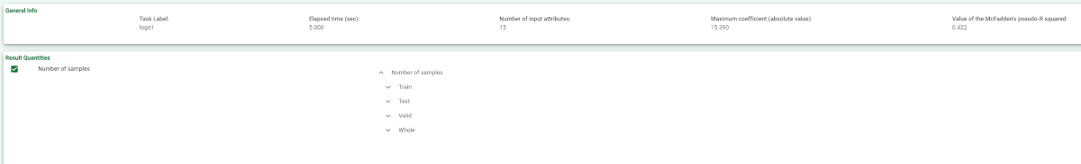 |
To check how the model built by Logistic model has been applied to our dataset, right-click the Apply Model task and select Take a look. Two result columns have been added:
| 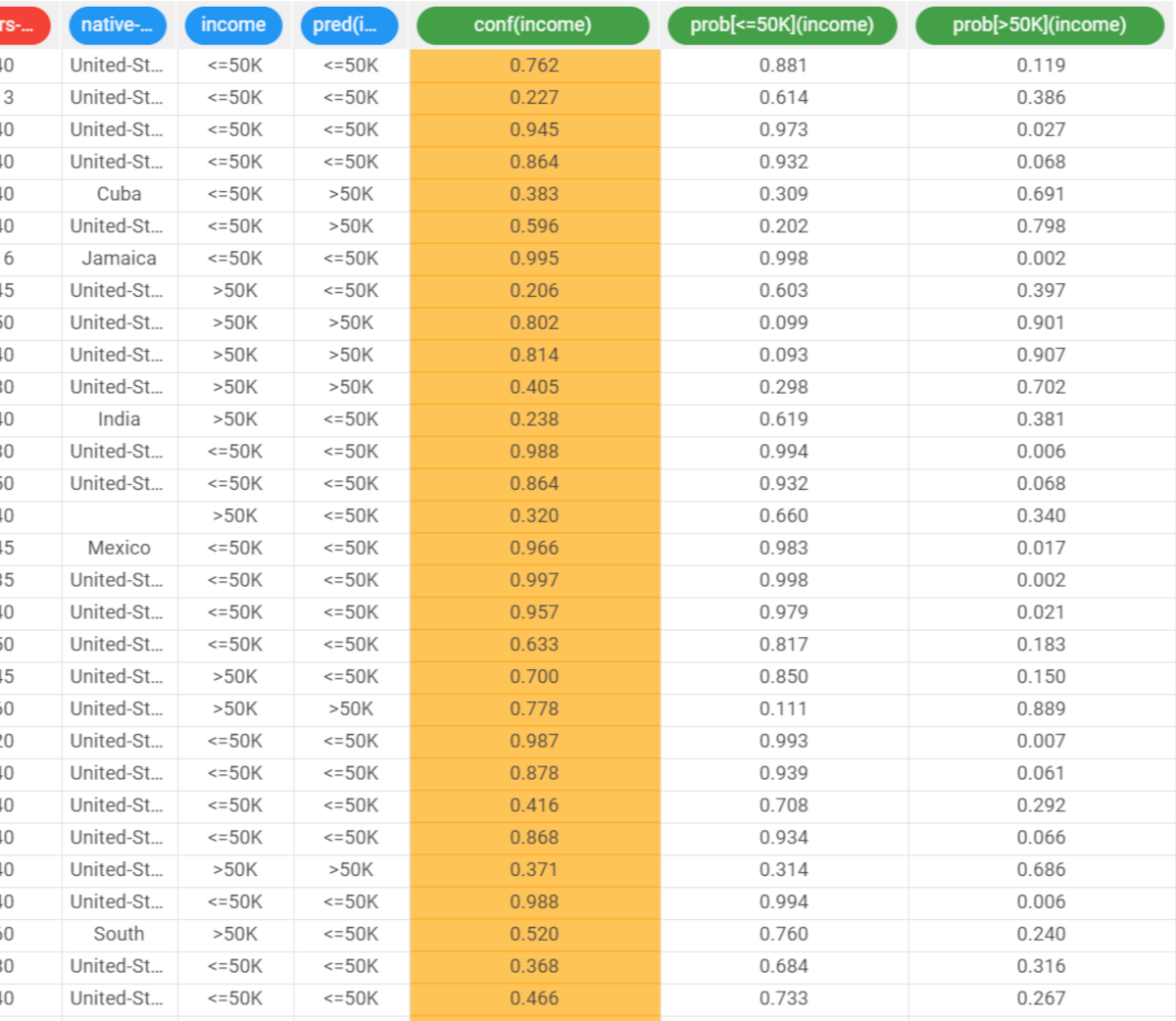 |