Using Linear to solve Regression Problems
The Linear solves regression problems in which the output value is expected to be a linear combination of the input variables through the Ordinary Least Squares (OLS) method.
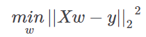
In mathematical notion, if ŷ is the predicted output value and 𝓍1,...,𝓍d the input variables, we want to find the weights vector 𝓌0,𝓌1,...,𝓌d such that ŷ=𝓌0+𝓌1𝓌1+...+𝓌d𝓍d.
The weights 𝓌1,...𝓌d are called coefficients, while 𝓌0 is the intercept or constant term.
Weights are computed in order to minimize the residual sum of squares between the input patterns in the dataset, and the responses predicted by the linear approximation. Mathematically this task solves a problem in the form:
The output of the task is the weights vector 𝓌0,𝓌1,...,𝓌d.
Prerequisites
you must have created a flow;
the required datasets must have been imported into the flow;
the data used for the analysis must have been well prepared, and contains a discrete or continuous output and a number of inputs;
a unified model must have been created by merging all the datasets in the flow.
Additional tabs
the Results tab, where statistics such as the execution time, number of attributes etc. are displayed.
the Coefficients tab, where the weight vector 𝓌1 relative to the Linear approximation is shown. Each element of the array is the coefficient of a single input attribute in the linear combination.
Procedure
Drag the Linear task onto the stage.
Connect a task, which contains the attributes from which you want to create the model, to the new task.
Double click the Linear task.
Drag and drop the input attributes, which will be used for regression, from the Available attributes list on the left to the Selected input attributes list.
Drag and drop the integer and/or continuous output attributes, which will be used for regression, from the Available attributes list on the left to the Selected output attribute list.
Configure the options described in the table below.
Save and compute the task.
Linear regression options | |
Parameter Name | Description |
|---|---|
Input attributes | Drag and drop here the input attributes you want to use to form the rules leading to the correct classification of data. Instead of manually dragging and dropping attributes, they can be defined via a filtered list. |
Output attributes | Drag and drop here the attributes you want to use to form the final classes into which the dataset will be divided. Instead of manually dragging and dropping attributes, they can be defined via a filtered list. |
Normalization of input variables | The type of normalization to use when treating ordered (discrete or continuous) variables. Possible methods are:
Every attribute can have its own value for this option, which can be set in the Data Manager task. These choices are preserved if Attribute is selected in the Normalization of input variables option; otherwise any selections made here overwrite previous selections made.
Normalization types For further info on possible types see Managing Attributes in the Data Manager. |
Normalization for output attributes | Select which method should be adopted to normalize output variables. Possible types are the same as those provided for input variables. |
P-value confidence | The p-value confidence value. |
Weight attribute | If specified, this attribute represents the relevance (weight) of each sample (i.e., of each row) with respect to the regression procedure. |
Regularization parameter | |
Value for constant term | If required, you can impose a value for the constant term which will be used to compute the coefficients. A value can be entered here if the Set value for constant term check box has been selected. |
Set value for constant term | If selected, you can enter a value in Value for constant term, which will be used to compute coefficients |
Aggregate data before processing | If selected, identical patterns are aggregated and considered as a single pattern during the training phase. |
Initialize random generator with seed | If selected, a seed, which defines the starting point in the sequence, is used during random generation operations. Consequently using the same seed each time will make each execution reproducible. Otherwise, each execution of the same task (with same options) may produce dissimilar results due to different random numbers being generated in some phases of the process. |
Append results | If selected, the results of this computation are appended to the dataset, otherwise they replace the results of previous computations. |


Example
The following example uses the Adult dataset.
Description | Screenshot |
|---|---|
| 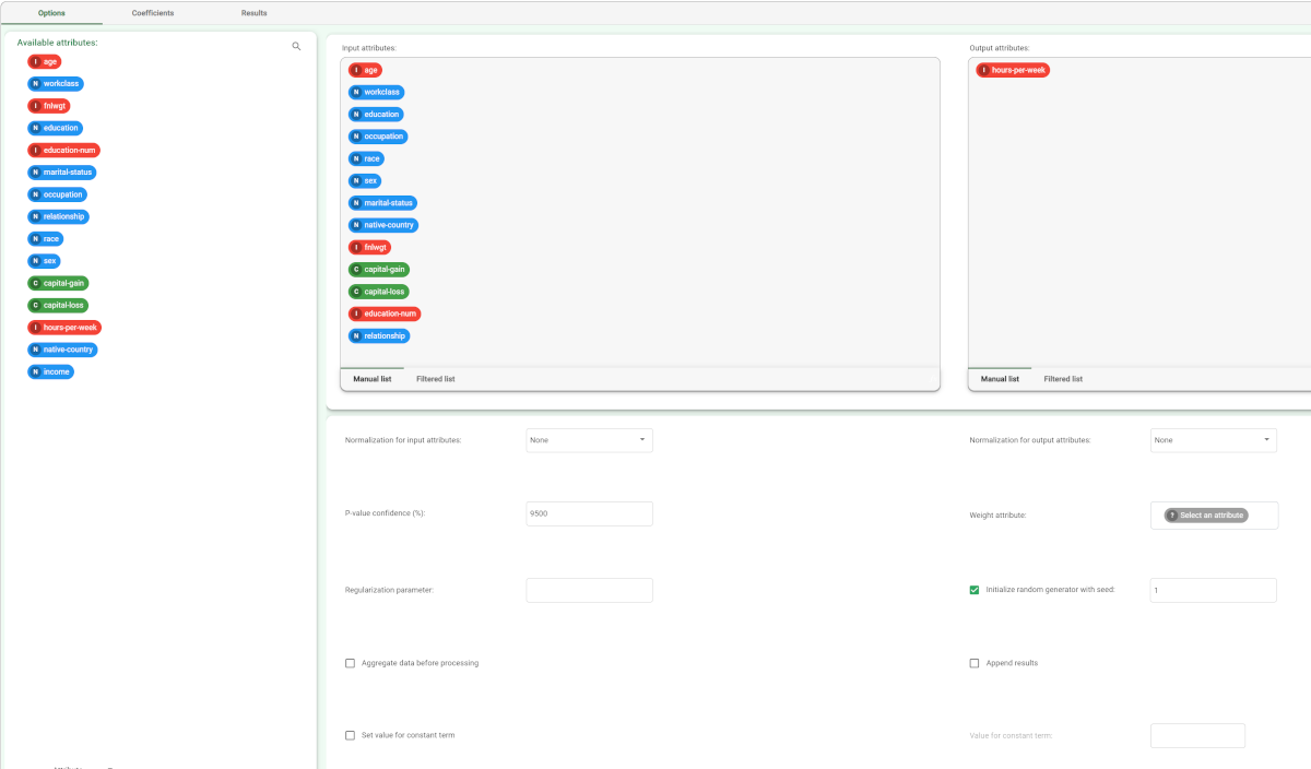 |
To check how the model built by Linear has been applied to our dataset, add a Data Manager to the flow. The Apply Model task has added two result columns:
| 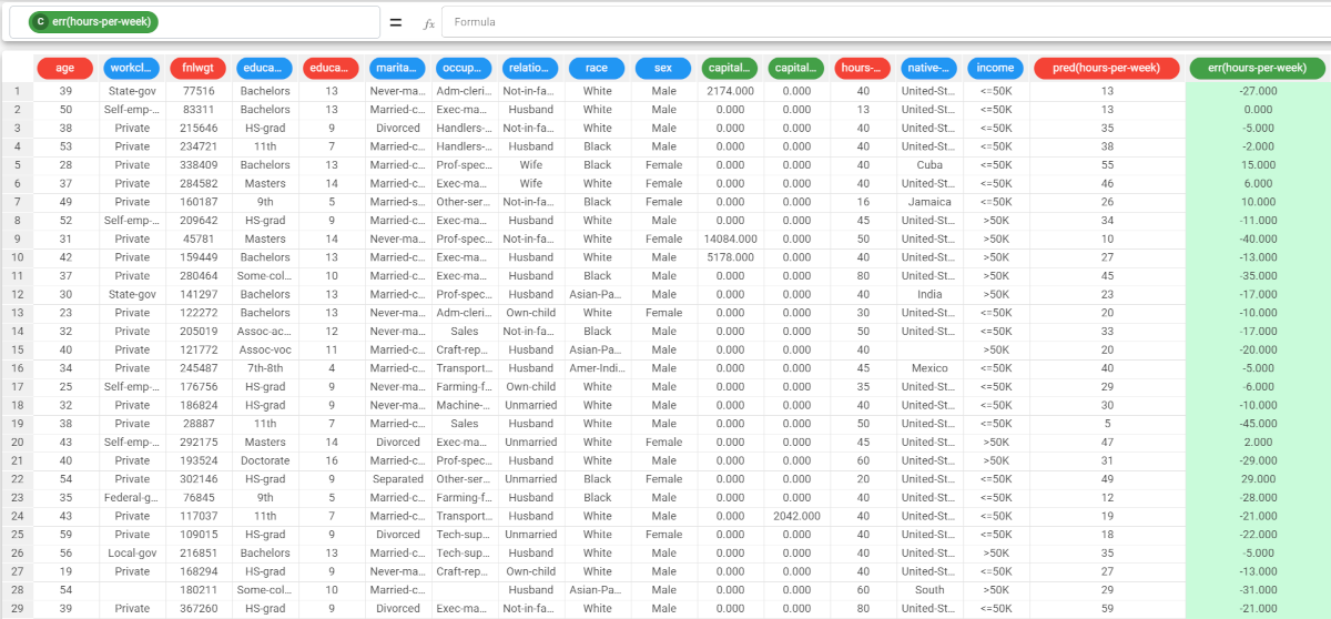 |