Using K-Nearest Neighbor to solve Regression Problems
The K-Nearest Neighbor (KNN) regression task determines the output of a new example on the basis its nearest neighbors.
In particular, given an input vector x, the algorithm finds its k nearest neighbors and then assigns x to the average of the output computed in this subset of examples.
The output of the task is a structure that can be employed by an Apply Model task to perform KNN forecasts on a set of examples.
Prerequisites
you must have created a flow;
the required datasets must have been imported into the flow;
the data used for the analysis must have been well prepared;
a unified model must have been created by merging all the datasets into the flow.
Additional tabs
The results of the K-Nearest Neighbor task can be viewed in two separate tabs:
The Points tab, where it is possible to view the points employed to perform the KNN classification. If no aggregation is performed and no attributes are ignored, this corresponds to the training set table. However, in many cases this table significantly differs from the training set and is therefore shown separately.
The Results tab, where statistics on the KNN computation are displayed, such as the execution time, number of points etc..
Procedure
Drag and drop the K-Nearest Neighbor task onto the stage.
Connect a task, which contains the attributes from which you want to create the model, to the new task.
Double click the K-Nearest Neighbor task.
Configure the options described in the table below.
Save and compute the task.
K-Nearest Neighbor options | |
Parameter Name | Description |
|---|---|
Input attributes | Drag the input attributes you want to use to build the network. |
Output attributes | Drag the output attributes you want to use to build the model. |
Normalization of input variables | The type of normalization to use when treating ordered (discrete or continuous) variables. Possible methods are:
Every attribute can have its own value for this option, which can be set in the Data Manager task. These choices are preserved if Attribute is selected in the Normalization of input variables option; otherwise any selections made here overwrite previous selections made. |
Normalization for output variables | The type of normalization to use when treating ordered (discrete or continuous) variables. Possible methods are:
Every attribute can have its own value for this option, which can be set in the Data Manager task. These choices are preserved if Attribute is selected in the Normalization of input variables option; otherwise any selections made here overwrite previous selections made. |
Aggregate data before flowing | If selected, identical patterns are aggregated and considered as a single pattern during the training phase. |
Initialize random generator with seed | If selected, a seed, which defines the starting point in the sequence, is used during random generation operations. Consequently using the same seed each time will make each execution reproducible. Otherwise, each execution of the same task (with same options) may produce dissimilar results due to different random numbers being generated in some phases of the flow. |
Append results | If selected, the results of this computation are appended to the dataset, otherwise they replace the results of previous computations. |


Example
The following example uses the Adult dataset.
Description | Screenshot |
|---|---|
Note that this regression problem in completely different from the KNN classification problem, where income was the output. In this regression example, we are not particularly interested in the physical meaning of this analysis, but only want to illustrate the potentiality of regression in a real-world dataset. | 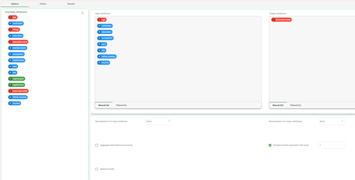 |
The Points table in K-Nearest Neighbor task contains the points (generated from the training set after an aggregation procedure) that will be used to perform the KNN regression operation. | 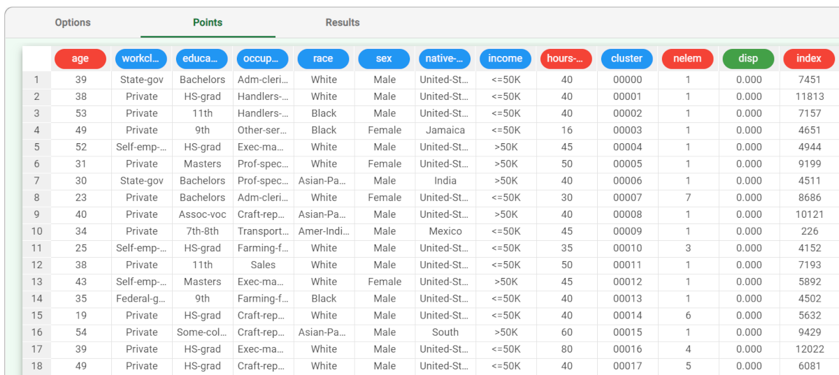 |
The forecast ability of the set of generated rules can be viewed by adding an Apply Model task to the K-Nearest Neighbor Regression task, and computing with default options. In the Apply Model task it is possible to select the number of nearest neighbors to be considered (i.e. the value of k): in this case we will select k=5. | 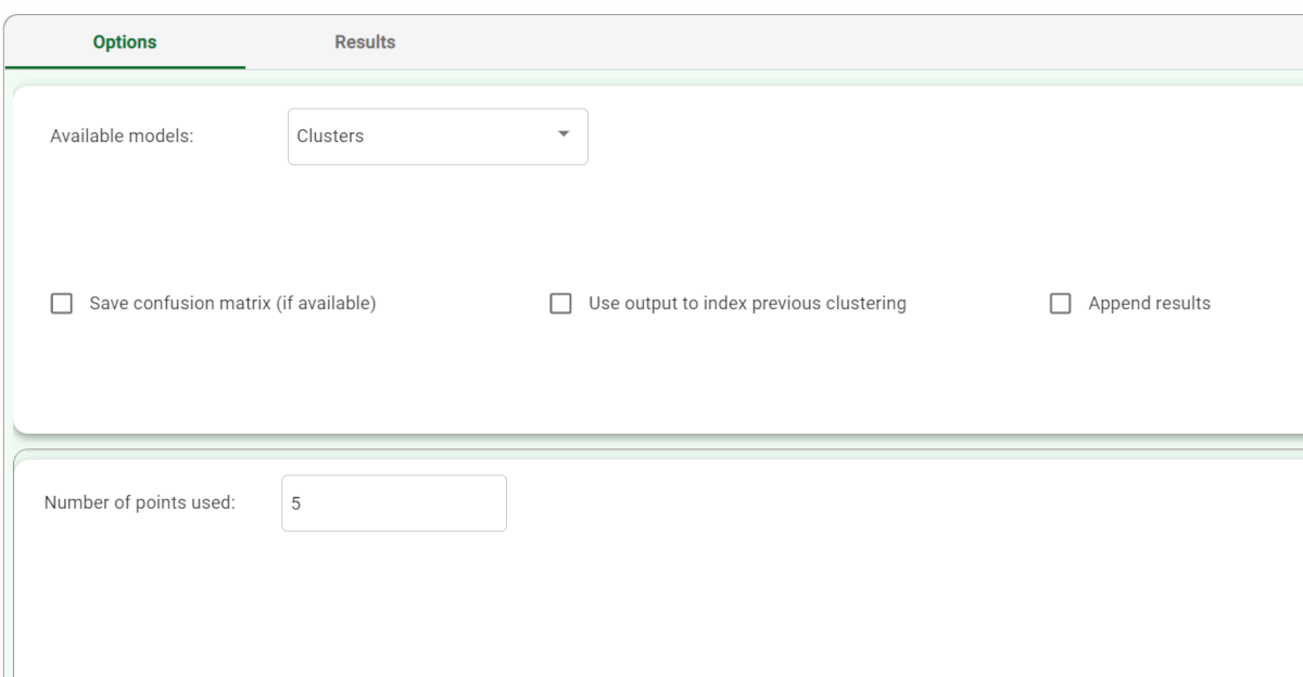 |
We can evaluate the accuracy of the model on the available examples by right-clicking the Apply Model task and selecting Take a look. The application of the rules generated by the KNN task has added four columns containing:
| 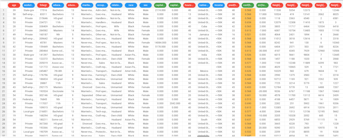 |