Decision Tree options

Input attributes

Drag and drop the input attributes which will be used to classify data in the decision tree.

Output attributes

Drag and drop the attributes which will be used to form the final classes into which the dataset will be divided.

Minimum number of patterns in a leaf

The minimum number of patterns that a leaf can contain. If a node contains less than this threshold, tree growth is stopped and the node is considered a leaf.

Maximum impurity in a leaf

Specify the threshold on the maximum impurity in a node. The impurity is calculated with the method selected in the Impurity measure option.

By default this value is zero, so trees grow until a pure node is obtained (if possible with training set data) and no ambiguities remain.

Pruning method

The method used to prune redundant leaves after tree creation. The following choices are currently available:

• No pruning: leaves are not pruned and the tree is left unchanged.

• Cost-complexity: according to this approach, implemented in CART the tree is pruned through a cost-complexity measure that creates a sequence of sub-trees and finds the best one through the application on a validation set. Each sub-tree is created from the previous one by minimizing a cost-complexity measure that takes into account both the misclassification level in the training set and the number of leaves.

• Reduced error: this simple method, introduced by Quinlan, employs the validation set to decide whether a sub-tree should be replaced by a single leaf. If the error in the validation set after transforming an internal node into a leaf decreases, the relative sub-tree is removed.

• Pessimistic (default choice): the tree is based according to the pessimistic pruning approach introduced by Quinlan. Using this method it is not necessary to create a validation set since the training set is employed both for tree creation and for tree pruning. Pessimistic pruning makes use of a a correction for the error rate (pessimistic error) at each node to decide whether it is to be pruned or not.

Method for handling missing data

Select the method to be used to handle missing data:

• Replace with average: missing values are replaced with the value fixed by the user for the corresponding attribute (for example, by means of a Data Manager). If this value is not set, the average computed on the training set is employed.

• Include in splits: patterns with missing values in the test attribute at a given node are sent to both the sub-nodes deriving from the split.

• Remove from splits: patterns with missing value in the test attribute are removed from the subsequent nodes.

Impurity measure

The method used to measure the impurity of a leaf. Considering a classification problem with c classes and a given node η, the following choices are currently available:

• Entropy, given by 

  

   where P_η(y_j) is the frequency of the j-th class in the node η.

• Gini, given by 

  

• Error, given by 

  

Initialize random generator with seed

If selected, a seed, which defines the starting point in the sequence, is used during random generation operations. Consequently using the same seed each time will make each execution reproducible. Otherwise, each execution of the same task (with same options) may produce dissimilar results due to different random numbers being generated in some phases of the process.

Select the attribute to split before the value

If selected, the QUEST method is used to select the best split. According to this approach, the best attribute to split is selected via a correlation measure, such as F-test or Chi-Square. After choosing the best attribute, the best value for splitting is selected.

Append results

If selected, the results of this computation are appended to the dataset, otherwise they replace the results of previous computations.

Aggregate data before processing

If selected, identical patterns are aggregated and considered as a single pattern during the training phase.

After importing the adult dataset with the Import from Text File task and splitting the dataset into test and training sets (20% test, 20% validation and 60% training) with the Split Data task, add a Decision Tree task to the process and double click the task.

Select:

• Cost-complexity as pruning method

• 0.5 as Maximum impurity in a leaf

• Income as the output attribute

Compute the task to start the analysis.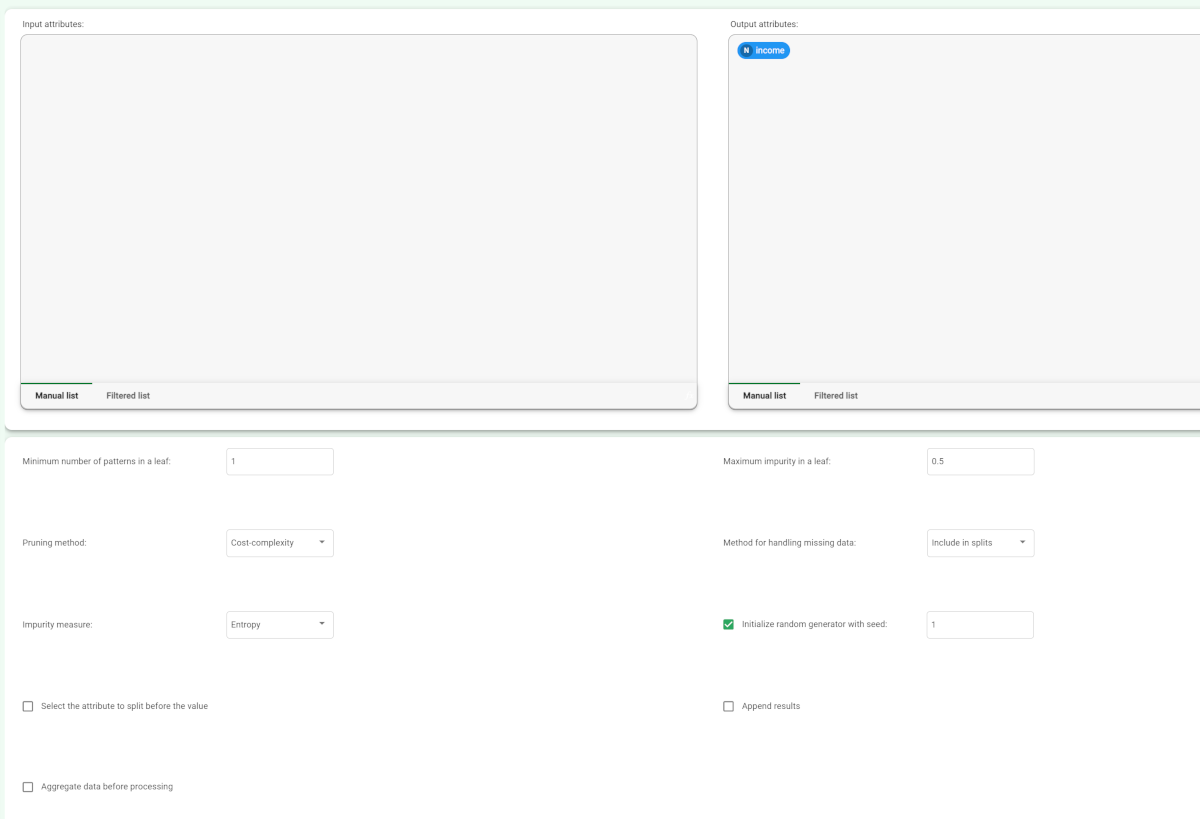

The properties of the generated rules can be viewed in the Monitor tab of the Decision Tree task: 

There are, for example, 656 rules with 4 conditions, 515 relative to class "<50K, and 141 relative to class “>50K”.

The total number of rules, and the minimum, maximum and average of the number of conditions is reported, too.

Analogous histograms can be viewed for covering and error, by clicking on the corresponding tabs.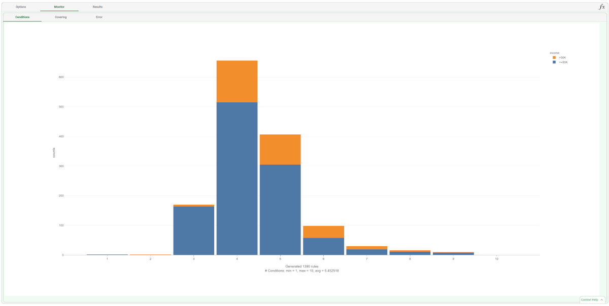

Clicking on the Results tab displays a spreadsheet with 

• the execution time (only for the DT task),

• some input data properties, such as the number of patterns and attributes

• some results of the computation, such as number of rules and rule statistics.

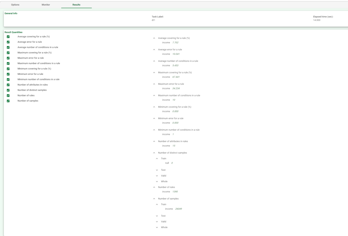The rule spreadsheet then can be viewed by adding a Rule Manager task.

Each row displays all the conditions that belong to the specific rule.

The total number of generated rules is 1390, with a number of conditions ranging from 1 to 10.

The maximum covering value is 67.4%, whereas the maximum error is about 15%.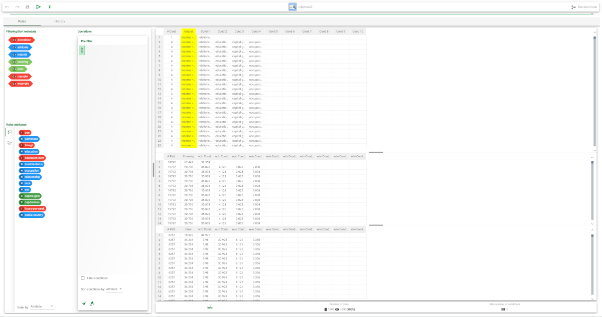

We can check out the application of this set of rules to the training and test patterns by right-clicking the Apply Model task and selecting Take a look.

The application of the rules generated by the Decision Tree task has added new columns containing:

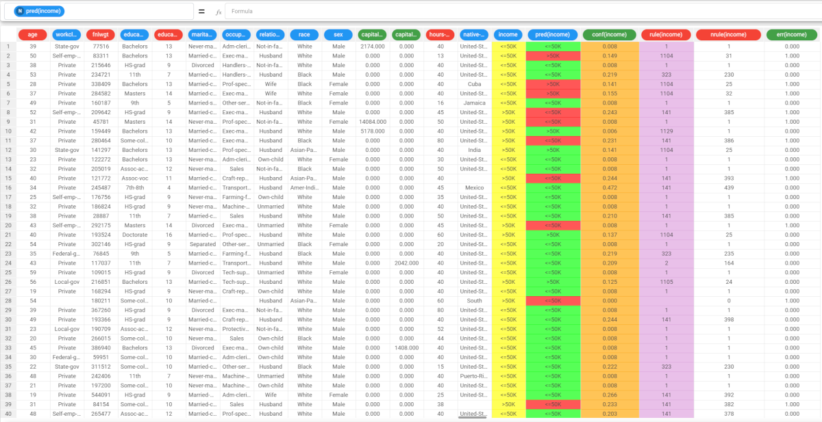• the forecast for each pattern: pred(income)

• the confidence relative to this forecast: conf(income)

• the number of rules used by each pattern rule(income)

• the most important rule that determined the prediction: nrule(income)

• the classification error, i.e. 1 if misclassified and 0 if correctly classified: err(income).