Using Mixed Integer Linear Programming to solve Optimization Problems
Linear programming is used to obtain the optimal solution for a problem by representing a real life scenario as a mathematical model with defined constraints.
Typical linear problems consist in finding the optimal values for a set of attributes (inputs) in order to minimize costs or maximize performance levels.
Rulex provides the Mixed Integer Linear Programming task, which means that:
the model and the constraints must be expressed as linear combinations of the inputs
the optimal values for the inputs can either be expressed as a rounded-up integer or as a continuous value.
Prerequisites
you must have created a flow;
the required datasets must have been imported into the process;
the input dataset must have the following structure:
a column with a label describing the contents of the row (objective function, constraints etc.)
a column for every variable included in the problem
a column containing the right hand side (constant term) of constraints
a row labeled with the objective function (valid strings are objective or cost)
a row for each constraint
optional rows with the minimum and/or maximum for each variable (by default 0 and infinite).
Procedure
Drag the Mixed Integer Linear Programming task onto the stage.
Connect the Mixed Integer Linear Programming task to the task which contains the data for the optimization model.
Double click the Mixed Integer Linear Programming task. The left-hand pane displays a list of all the available attributes in the dataset, which can be ordered and searched as required.
Configure the options as described in the table below.
Save and compute the task.
Mixed Integer Linear Programming options | |
Parameter Name | Description |
|---|---|
Table Mode | Choose one of the following:
Once the Table Mode is chosen, the task will change its layout according to it. |
Normal Table Mode options | |
Coefficients for integer solution | Drag and drop from the Available attributes list the coefficient attributes that will be used in the calculation, if the results must be provided as an integer. Instead of manually dragging and dropping attributes, they can be defined via a filtered list. Note that the type of the associated coefficient attribute is independent from the type of the result you want to obtain. |
Coefficients for continuous solutions | Drag and drop from the Available attributes list the coefficient attributes that will be used in the calculation, if results can be provided as a continuous value. Instead of manually dragging and dropping attributes, they can be defined via a filtered list. Note that the type of the associated coefficient attribute is independent from the type of the result you want to obtain. |
Attribute for constraint (and cost) types | Select the attribute (column) which contains the row type, which can be:
|
Attribute for right hand side values | Select the attribute (column) that contains the constants for the constraint rows. |
Sparse Table Mode options | |
Attribute for row value | Select the attribute containing a label to identify which constraint you are referring to. Its type can be both ordinal or nominal. |
Attribute for col value | Select the attribute containing the output attribute’s name. Its type can be both ordinal or nominal. |
Attribute for coefficient value | Select the attribute containing the coefficient used to make the analysis. |
Shared options between both table modes | |
Optimization mode | Select whether you want your solution to Maximize or Minimize the outcome. |
Maximum execution time | Specify for how many seconds the task can run. If not specified, no time limits are set. |
Maximum number of iterations | Specify how many times the task can be run. If not specified, no limits on the number of iterations are set. |
Results
The results of the task can be viewed in two separate tabs:
The Solution tab displays the generated solutions. The tab will display the results only if you have not selected the Overwrite data with solution coefficients option.
The Results tab, where information on the task execution is displayed, such as the elapsed time.
Example
The following example uses the yogurt dataset.
The basic scenario used in this example involves a small family-run farm factory where two types of yogurt are produced:
deluxe strawberry yogurt, which contains two units of yogurt and two units of strawberries, and produces a profit of 3 euros per unit of finished yogurt.
super saver yogurt, which contains three units of yogurt and one unit of strawberries, and produces a profit of 2 euros per unit of finished yogurt.
There are currently 15 units of yogurt and 10 units of strawberries in stock, and at least two units of each type of yogurt must be produced to meet current orders.
Objective: The factory wants to maximize its profits by finding out the optimal amount of deluxe and super saver yogurt to make with its currently available stock.
The information in the scenario can be mathematically expressed as follows
The amount of deluxe yogurt to produce = x
The amount of saver yogurt to produce = y
The maximum profit = z
Consequently z = 3x (profit multiplied by the amount produced) + 2y
Our constraints are as follows:
Strawberry stock constraint: 2x + y <= 10
Yogurt stock constraint: 2x + 3y <= 15
Minimum values:
x >=2
y >=2
Description | Screenshot |
|---|---|
| 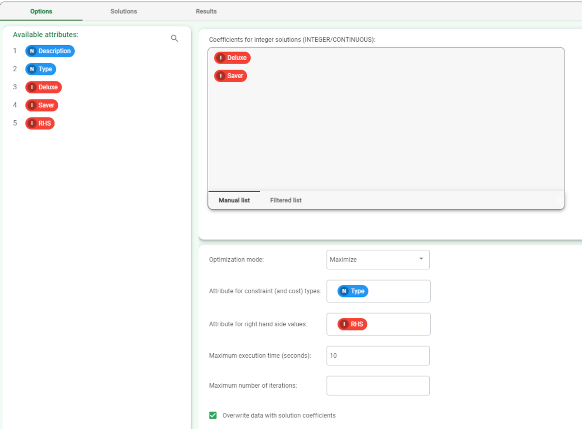 |
After saving and clicking Compute to start the analysis, the solution to our problem can be viewed in the Data Manager task. The maximum profit is 16 euros (objective), if we produce (and obviously manage to sell):
| 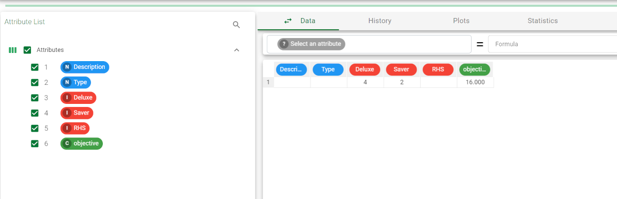 The same information can be viewed directly in the Solutions tab of the Mixed Integer Linear Programming task if we do not select Overwrite data with solution coefficients. |