Plotting Stat Plots in the Data Manager
Stat Plots have no relation with the other plots available in the Data Manager, as they display statistical analysis.
You can choose between the following plots:
Plot | Description |
|---|---|
ROC Curve (default) | It illustrates the performance of a binary classifier system as its discrimination threshold is varied. |
Lorenz Curve | It is a graphical representation of the Lorenz distribution, which is often associated with the distribution of wealth among the population, according to the Gini Index. |
P-P Plot | It is a probability plot used to evaluate if a data set follows some specified distribution, plotting the two cumulative function against each other. |
Q-Q Plot | It is a probability plot used to compare two probability distributions by plotting their quantiles against each other. If the two distributions being compared are similar, the points in the Q-Q plot will approximately lie on the line y = x. In a Q-Q plot it is possible to compare two empirical probability distribution or an empirical one with a standard probability distribution. |
Plot elements
When building a Stat Plot, you need to provide the required elements, which change according to the plot type.
Plot elements | ||
|---|---|---|
Element | Mandatory | Constraints |
X | Yes (all plots) |
|
Y | Yes (Q-Q Plots only) | It cannot be a nominal value. |
TARGET | Yes (ROC Curve only) | |
Prerequisites
you must have created a flow;
you must have linked the Data Manager to the task which contains the data to work on.
Procedure
In the Plots tab of the Data Manager, click on the plus button to add a new plot.
Select the plot type and choose the Stat Plot. A ROC Curve is created by default.
Switch the plot type by right-clicking onto the Stat Plot icon.
Drag the required attributes onto the plot elements.
If required, work on the attributes on the plot, for example to modify their values.
Configure the plot options, if required, by right-clicking on the single plot elements' icons.
Hover over the plot to view its details. The details change according to the plot type.
Modify the display options, if required.
Click on the wrench button to configure the overall layout settings.
Save and compute the task.
Customization constraints If you drag a second attribute on an element of an existing plot, the first attribute is replaced by the new one; If you drag a second attribute on an element of an existing plot, hold down the CTRL button on your keyboard when dropping the second attribute to create another plot with the new attribute on the chosen element. If you drag a second attribute on an element of an existing plot, hold down the SHIFT button on your keyboard when dropping the second attribute to add the second attribute to the same plot, so that one element will contain two attributes. To know more about the plot’s elements, go to the Elements page.
You can decide to separate the attributes onto two different plots, by right clicking on the attribute and selecting Detach. If you want to merge the two attributes again, right click on the second attribute and select Attach.
Example
The following example uses the customers dataset.
Description | Screenshot |
|---|---|
Add a new plot, and choose the Stat Plot. Drag the Number of operations last year attribute onto the X axis and the Job attribute onto the TARGET area. Once the Number of operations last year attribute is dragged onto the X axis, the TARGET icon becomes red, as it is a mandatory parameter. Continue building the plot. | 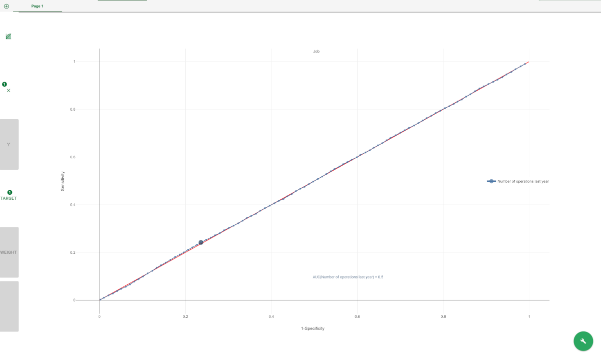 |
Switch between the Stat Plots available by right clicking onto the plot type icon and choosing the required plot in the drop down lists available, then click Apply. | 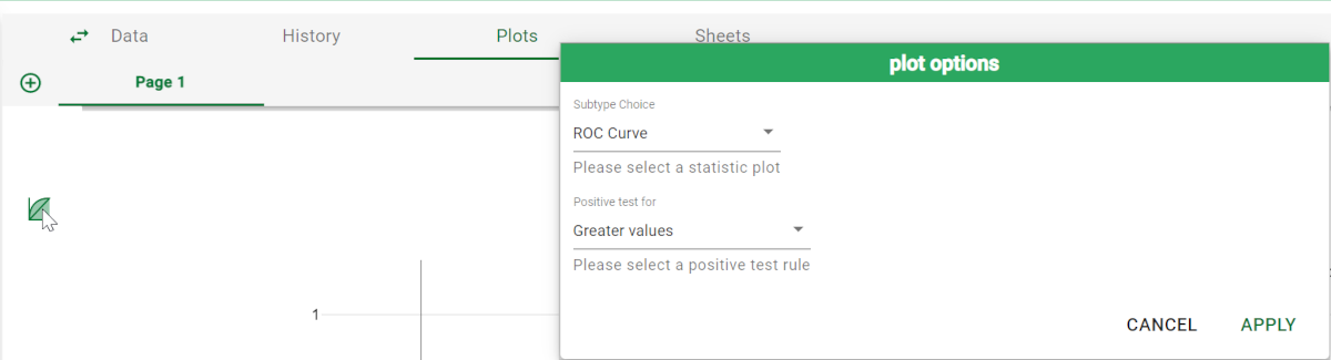 |