Discretizing Data
Discretization transforms continuous data by defining a set of cutoffs that subdivide a continuous domain into a finite set of homogeneous intervals.
The points in each interval should have a high probability of belonging to the same class. These intervals increase the effectiveness of data in the creation of predictive models.
Prerequisites
you must have created a flow;
the required datasets /wiki/spaces/RPDP/pages/2658467884into the flow.
Procedure
Drag the Discretize task onto the stage.
Connect a task that contains the attributes you want to transform to the Discretize task.
Double click the Discretize task. On the left hand side of the pane there is a list of all the available attributes in the dataset, which can be ordered and searched as required.
Configure the options, as described in the table below.
Save and compute the task.
Discretize options | |
Name | Description |
|---|---|
Use previous cutoffs to discretize dataset | If selected, the cutoffs defined in an upstream Discretize task will be used to discretize the new data, instead of defining new cutoffs. This is useful when you want data to be discretized in the same way in various point of the worklflow. |
Attributes to discretize | Drag and drop the ordered attribute you want to transform from the Available attributes list. |
Method for discretization | Select the method you want to use from the Method for discretization drop-down list. Possible values are:
The Attribute Driven Incremental Discretization method usually scores the best performance but may be quite time consuming when there are large training sets. The Entropy method is usually faster but may generate some ambiguities and then compromise the accuracy of any subsequent analysis.
|
Minimum distance between different classes | Specifies the minimum distance that must be kept between two patterns of different classes, as the percentage of the total number of attributes. This distance is computed as the number of attributes whose values are different in the two patterns. The minimum and default distance is one. If you select 100% all the attributes of each couple of heterogeneous patterns must differ. This is not always possible since many attribute can have the same value in the starting data, and in this case the method uses the available separations. |
Output attribute | Select the output attribute to be used for discretization from the drop-down list. Output attributes are mandatory for supervised methods. |
Number of patterns used for discretization | Specifies how many patterns will be used. This option allows you to use only a randomly selected subset of the training set, which is particularly useful when there is a high amount of data, as a high number of patterns considerably slows sown the discretization process. The default value of -1 means that all patterns will be used. |
Number of values for ordered variables | Specifies the number of cutoffs to be inserted for each variable, which must not exceed the number of values available in the training set. The number of cutoffs must at least ensure that the minimum distance between different classes can be guaranteed. |
Preselect best cutoffs | If selected, the most promising cutoffs will be selected and employed in the subsequent phase. This consequently reduces the number of possible cutoffs to be analyzed. This works particularly well coupled with the Attribute Driven Incremental Discretization method. |
Aggregate data before processing | If selected, identical patterns will be aggregated and considered as a single pattern during the discretization phase. |
Discretize output | If selected the output attribute will be discretized. This option is available if you selected a discrete (e.g. integer) or continuous output attribute. You can then select the required discretization method in the Discretization method for output option.
|
Discretization method for output | Select the discretization method you want to adopt to discretize the output. This option is available only if you have selected the Discretion output option. Possible methods are:
|
Number of cutoffs for output | Select the number of intervals to be created when discretizing output values. The default is 10 whereas 0 means that all possible cutoffs have to be inserted. This option is available only if you have selected the Discretize output option. |
Example
The following example uses the Adult dataset.
Description | Screenshot |
|---|---|
| 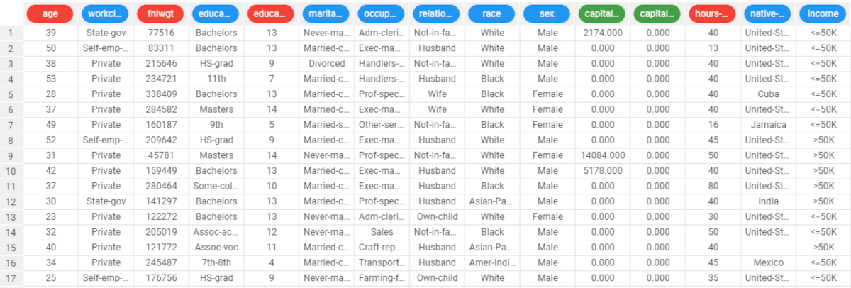 |
| 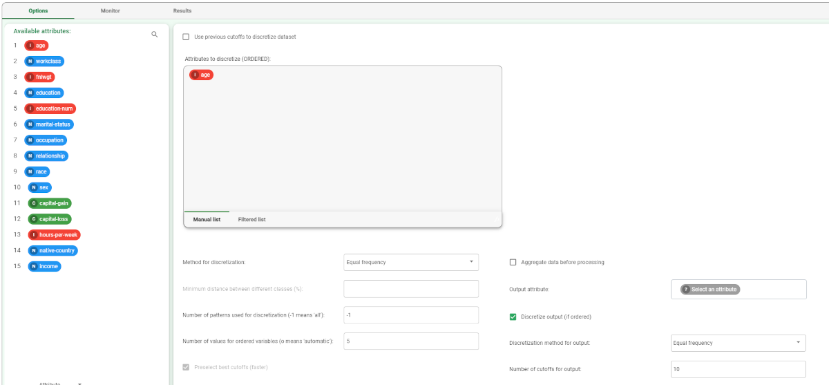 |
| 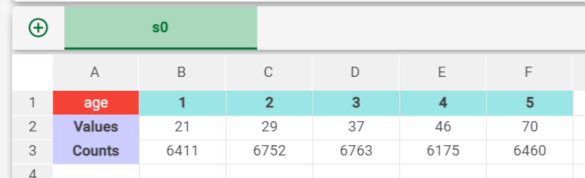 |